
How to Freeze Rows and Columns in Excel
How to Freeze Rows and Columns in Excel – Have you ever seen excel file where part of the rows or columns remain visible and don’t move when scrolling down or sideways? If you ever find one then that’s how the freeze row and column function in Excel works.
The Freeze Panes feature is available in almost all Excel versions including Office Excel 2007, Excel 2010, Excel 2013, Excel 2016, Excel 365 and Excel Online versions.
What is the freeze panes feature?
The Freeze Panes function is a feature that is used to freeze certain rows and or columns in an Excel worksheet or worksheet, so that when you shift the position of cells on the Excel worksheet, the row and / or column positions do not move and can still be seen.
In other words, if the Freeze Panes feature is active, when we scroll or shift the Excel worksheet, the position of Excel rows and or columns will not shift and remain locked.
How to use Excel Freeze Panes?
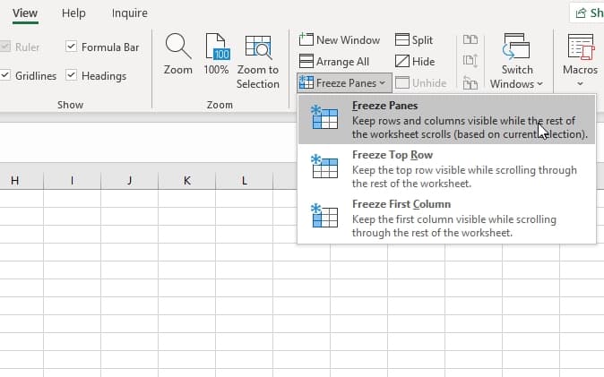
The Freeze Panes feature can be found in the View Tab – Freeze Panes as shown in the following image.
How to freeze the first row in Excel?
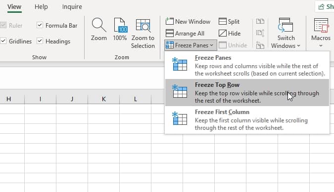
Make sure the position of the first row we are going to freeze is visible on the worksheet. Then, in the View Tab – Freeze Panes, select the Freeze Top Row menu
How to freeze the first column of Excel?
To lock the first column so that it doesn’t shift when we scroll to the right, the steps required are as follows:
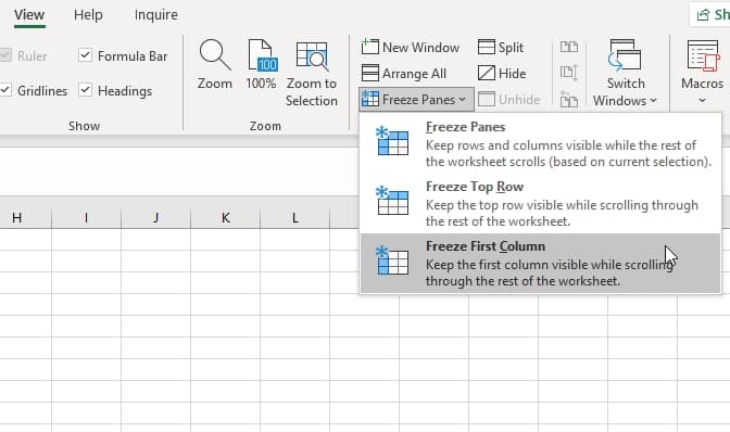
Make sure the position of the column that we will lock with Freeze panes is in the left position. In the View Tab – Freeze Panes, select the Freeze First Column menu.
How to freeze multiple excel lines at once?
With Freeze Top Row, only the top row will be frozen or locked when scrolling the Excel worksheet. Then how to freeze multiple rows (Rows) in Excel?
To Freeze Panes more than one line in Excel, the steps required are as follows:
- Select the row that is below the bottom row that you will freeze. An easy way is to click the row number on the row number of the Excel worksheet. For example, if you are going to lock rows 1-4 so that it doesn’t move when scrolling, then select or mark all cells in row 5.
- Then on the View Tab – Freeze Panes select the Freeze Panes menu.
Well, it’s easy right? In the example above, after Freeze Panes, lines 1-4 will not move when we scroll. Then what about Freeze Panes for multiple columns?
How to Freeze More Than One Excel Column
How to Freeze multiple Excel columns at once? With Freeze First Column, only the leftmost excel column will be locked from shifting to the right. So how to freeze panes for more than one column the ways you can do are as follows:
- Select the column that is to the right of the rightmost column of the several columns that you will lock. The trick is to click on the column name at the top. For example, if you are going to lock columns A through C then select or mark all columns D.
- Then on the View Tab – Freeze Panes, then please select the Freeze Panes menu. In the example above, after Freeze Panes is active, columns A, B and C will not move when we scroll.
The four methods above explain how to freeze one or more rows or columns only. Then how do you freeze panes on Excel columns and rows simultaneously? Follow this next excel freeze method to freeze or lock columns and rows at once in excel.
How To Freeze Columns And Rows Simultaneously
How to Freeze columns and rows at once in Excel? How to freeze columns and rows at once or freeze columns and rows simultaneously in Excel is very easy. here are the steps:
- Select the cells that are below the bottom row as well as the cells that are to the right of the rightmost column of the rows and columns that will be frozen together. For example, if you are going to freeze row number 3 and column C then position the cursor or active cell in cell D3.
- Then on the View Tab – Freeze Panes, please select the Freeze Panes menu.
How to UnFreeze Excel
How to get rid of freeze in Excel? If it is no longer needed or there is a position error when doing this Freeze Panes, you can deactivate or unfreeze this feature by selecting the Unfreeze Panes menu in the View Tab – Freeze Panes as shown in the following image. The Unfreeze Panes menu will only appear when Excel’s Freeze Panes feature is active.